Abstract
Starting from the Atlas repository, a Github repository by LiamHz, which procedurally generated terrain, our team worked together to make the visuals pop. Beginning with no OpenGL experience, over the course of a month in April, we implemented various user controls, fog effects, blending, skyboxes, grass instancing, and reflective and refractive water. We hope that you enjoy the visuals!
Technical Approach
Context and Where We Started From
Before delving into the technical details of our implementation, here's some relevant context about the original author's procedural terrain implementation.
- The terrain is generated in chunks. For example, a large map may be represented by a 10 x 10 grid, with each fixed grid size composed of a mesh chunk (a “terrain chunk”).
- A given terrain chunk is a single mesh, with varied colors to represent different surfaces such as water, grass, rock, and snow.
- The surfaces are classified (and colored) based on their height proportional to max height size.
- The world generation can be changed by providing different parameters relating to the Perlin noise and size of the map.
Fog
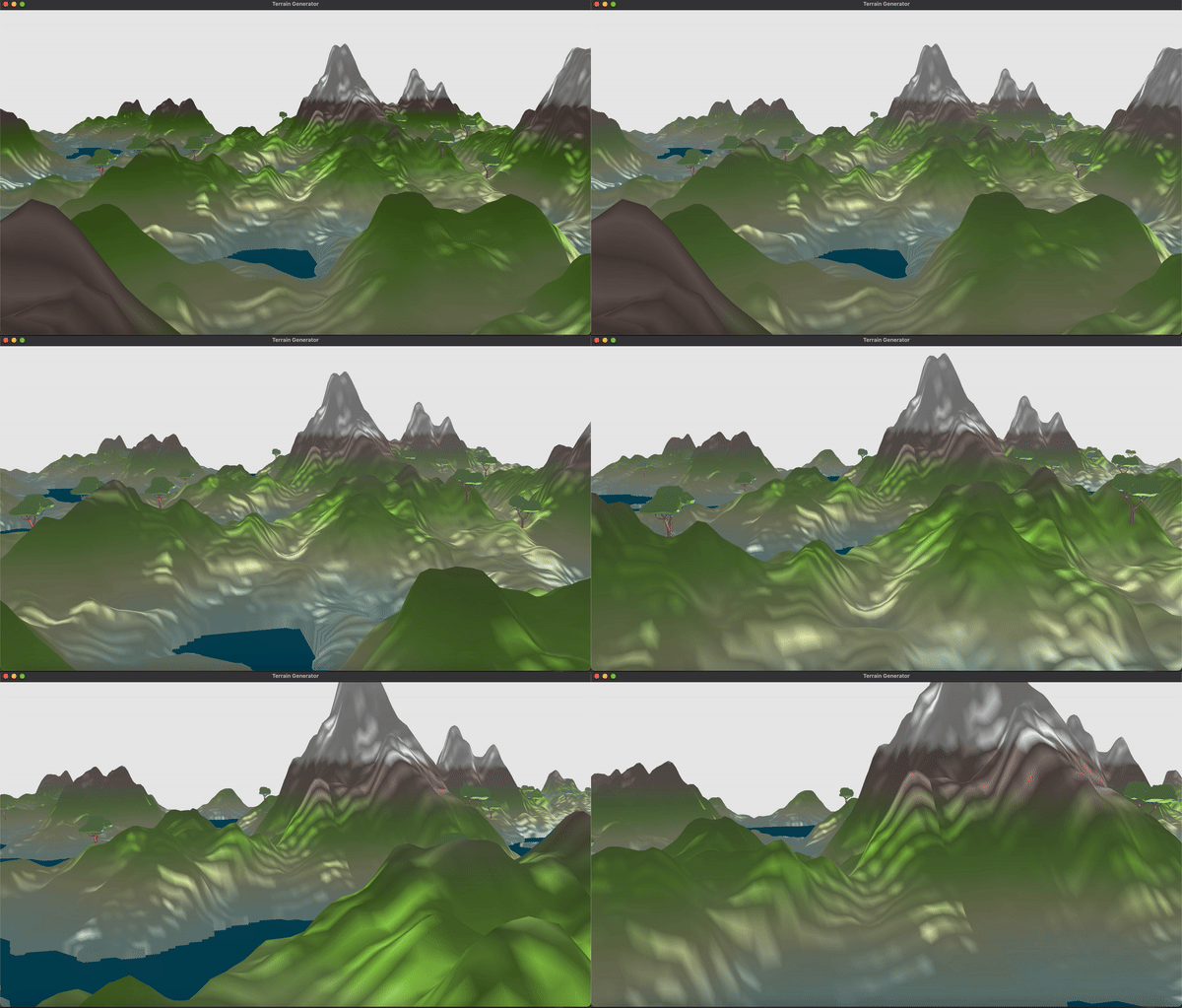
At a high level overview, fog is an environmental effect that interferes with the normal sight of line which would absorb and scatter the light rays reflected off of objects. This means that each of the vertices would need to be a mix of its current color as well as the fog color. Core fog parameters include the distance between each pixel and the camera, the fog color, as well as fog density. At farther distances, objects tend to “hide” behind the fog which would mean that the pixels would blend in more with the natural fog color instead of its original color. We defined a fog factor based on the distance away from the camera and it was 1 there would be no fog and would just be the pixel color while as the fog factor decreased to 0 the fog color would take over.
At first, we implemented a simple shader to render fog for our scene by blending the pixel color with the fog color via linear interpolation. This is referred to as “linear” fog and the fog factor was simply the ratio between the distance of the pixel to the camera over the entire rendering distance. Any pixels beyond the maximum rendering distance would get the color of the fog. Everything in between would be linearly interpolated. Thus, the fog factor is based on the ratio of the fragment to the camera to the chunk render distance. Here is the linear fog shader:
Then, we decided to build upon this linear fog with more advanced shading where the fog increases exponentially as we move away from the camera. This would create a more dramatic effect at a certain rendering distance as the objects become more fully immersed in the fog. The first formula for the fog factor we used was \(\frac{1}{e^{\text{distance} * \text{density}}}\). The density number is simply a way to tune the fog up or down. We used a similar approach from before to calculate the distance from the pixel to the camera. Finally, we used another approach for the fog factor which was \(\frac{1}{e^{(\text{distance} * \text{density})^2}}\). This would create an effect where closer to the camera there would be less fog but drops sharply and levels off as the distance increases. This gives a more natural feel as the fog is not as dominating closer to the camera compared to the exponential fog. Here is the exponential squared fog:
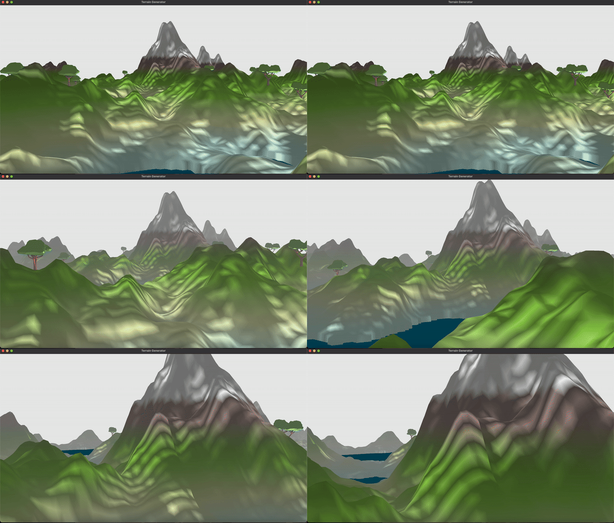
We combined each of these fog shaders into a single .frag and .vert files and created keyboard toggles to select the shader we wanted. The entire pipeline included getting the vertex position, normals, and colors from each pixel and then calculating the fog factor in the .frag file based on the distance and appropriate exponential function if necessary. Afterwards, based on this fog factor we would mix the pixel color and the fog color and use this as the new fragment color. If fog is not enabled, we set the fragment color as the original pixel color.
We ran into some issues with the fog implementation as initially the shader would make everything black. To debug, we pushed the newly calculated fog factors into the color to see what the output would be and realized that it was 0 and thus caused the black colors to appear. To fix this, we had to change what the passed in rendering distance was into the .vert file and we used the max between the width and height multiplied by the chunk distance as this was how far the camera was able to see. There were also some issues where the color would turn magenta and we noticed that the fog factor was greater than 1 so we had to clamp the fog factor. Through this trial and error, we learned how to debug in GLSL files to get what we needed.
Grass
Put simply, we created grass by criss-crossing 2D "billboards" at every vertex on our terrain where there should be grass, and texture mapping an image of grass blades onto the billboards while filtering out parts that weren't grass blades.
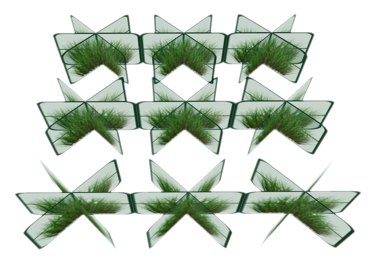
Step 1 was collecting the grass vertices. Outside of the render loop and on the CPU, we iterated through each chunk of the terrain and collected all vertices that corresponded to grass locations based on their height.
Step 2 was associating each chunk of terrain and grass vertices to a corresponding VAO (Vertex Array Object) and VBO (Vertex Buffer Object). VAOs and VBOs are OpenGL objects used for efficient rendering of vertex data. A VBO stores the actual vertex data (positions, normals, texture coordinates, etc.) in GPU memory. A VAO is a container that stores the state of how the vertex data in the VBOs should be interpreted and mapped to the vertex shader's input attributes. We created a VAO for each chunk and stored the corresponding grass vertex data in a VBO. This setup allowed us to render the grass vertices efficiently by simply binding the corresponding VAO before drawing.
Step 3 was the render loop and transformation matrices. For each frame, we computed a projection matrix, view matrix, and model matrix. The projection matrix defines the perspective projection transformation, which maps 3D coordinates from the camera's view space into 2D coordinates in the clip space (the visible region on the screen). We calculated it using glm::perspective, defining the perspective projection based on the camera's field of view, aspect ratio, and near/far clipping planes. The view matrix represents the transformation from world space to camera (view) space. It encodes the position and orientation of the camera in the world, essentially defining the camera's view. The model matrix represents the transformation from object (chunk) space to world space. Each chunk in our terrain has its own model matrix, which encodes its position and orientation in the world. More importantly, we sent all these matrices to our shader as uniform variables for it to access, and for each chunk within render distance, we bound its corresponding VAO and issued a command to glDrawArrays to draw all the VAO's corresponding vertices onto the screen.
Step 4, still inside the render loop or per frame computations, was the shaders. For each vertex that comes from glDrawArrays, OpenGL executes the vertex shader, passing the vertex data as input. Our vertex shader was simple; it simply lifted the vertex positions slightly above the surface to prevent the grass from being buried. These vertices were then passed to our geometry shader. The geometry shader is an optional stage that operates on primitives (points, lines, or triangles) and can generate new primitives. In our case, the geometry shader was responsible for creating the grass billboards. It generated a series of rectangular billboards by emitting new vertices and transforming them based on various factors, such as wind, randomness, camera distance, and grass size. Most importantly, it brought each vertex into the correct location on the screen by multiplying first by the model matrix, transforming the vertices from object (chunk) space to world space; next, it multiplied by the view matrix, transforming the vertices from world space to view (camera) space; lastly, it multiplied by the projection matrix, projecting the vertices from 3D view space onto the 2D clip space. The last part in the geometry shader was outputting the UV coordinates for the fragment shader to use, and these were simply the four normalized coordinates of each billboard that the geometry shader created. The fragment shader is executed for every pixel that needs to be rendered on the screen, and if the pixel is within one of the quads generated by our geometry shader, then the rasterizer will interpolate across the corresponding UV coordinates outputted by nearby billboard vertices and pass them to our fragment shader. In our fragment shader, we were working with a texture that was an image of grass blades with a transparent background. So our fragment shader sampled the color using the UV coordinates and checked if the sampled color had a low alpha value (high transparency), indicating a background pixel. If so, the fragment was discarded using the discard keyword; otherwise, the opaque grass color was output as the final fragment color.
In conclusion, we used vertex, geometry, and fragment shaders to create realistic-looking grass billboards on top of a terrain. VAOs and VBOs ensured efficient rendering of the grass vertex data, while the geometry shader performed the heavy lifting of generating and transforming the billboard geometry based on various factors like wind, randomness, and camera distance. The fragment shader then applied the final touches by texture mapping the grass blades and filtering out transparent areas. While we did follow and reference two tutorials, it was still a challenge to implement because our transformation matrices had to be different from theirs due to the unique environment we started with, along with many other subtleties. We learned a lot about OpenGL and the graphics processing pipeline through this feature implementation and gained more appreciation for the even better looking grass that is commonly found in video games.
Snowy Grass
Our snowy grass takes a lot of inspiration from the regular grass. Although the texture is different, the shader is very similar. The most significant change was making the snowy grass render sparsely with a set probability for a more realistic appearance.
Water
As an overview, our implementation of water can be summarized by a plane, distortions, and texture mapping.Positioning
At the start, water was represented in the terrain by blue portions of the terrain mesh. The first step to enhancing the world's representation of water includes creating a water mesh separate from the large terrain mesh, allowing us to incorporate custom shaders. However, the locations of water are only known after program startup. Since a given terrain location is classified by height, we can post-process the generated terrain vertices to identify where the water should be.
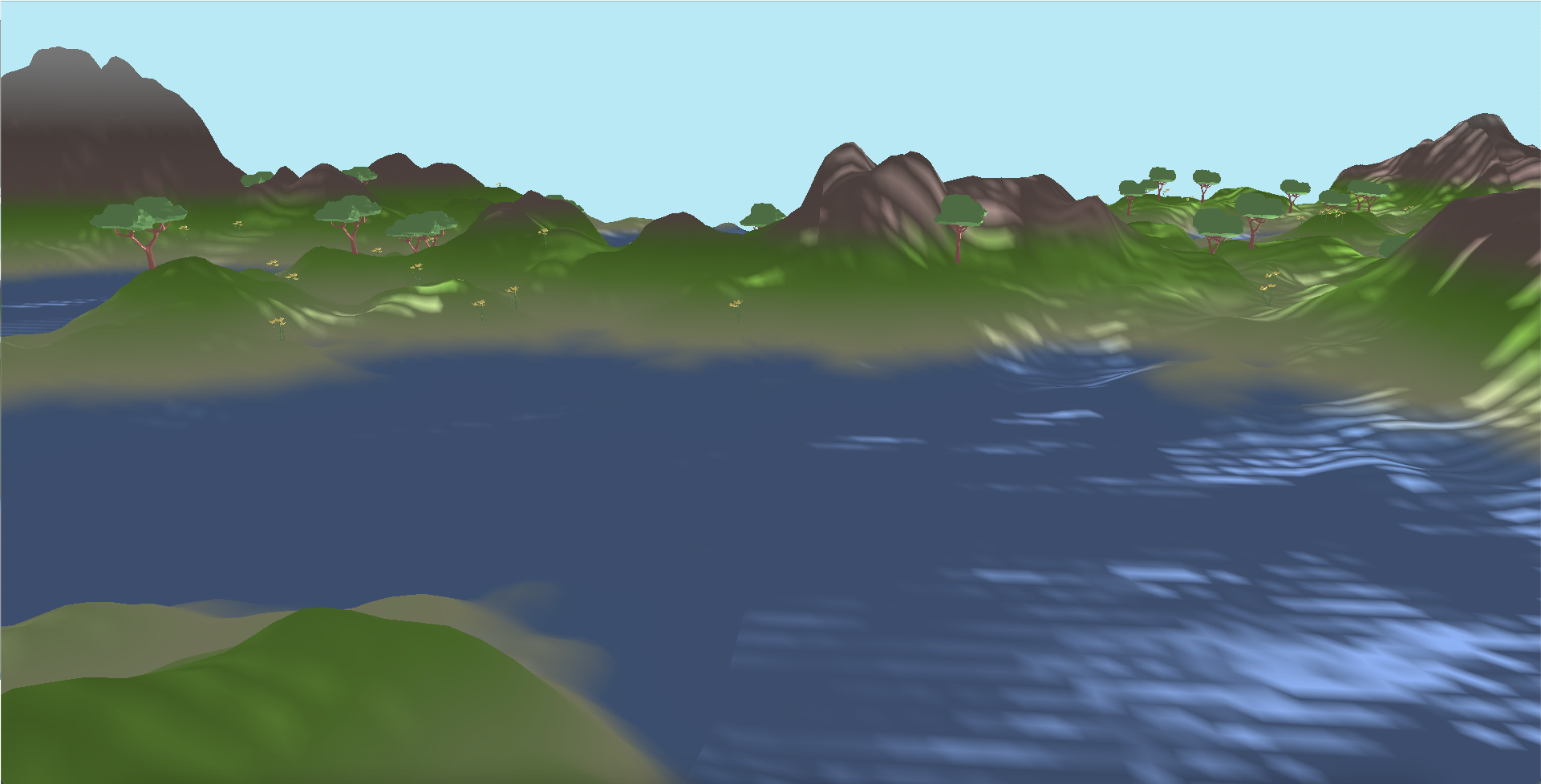
After determining the general location of the water, how do we actually create the water? There are a couple options, one of which is a single plane that runs through the whole mesh (as displayed in our milestone), while a second, more efficient option would be to find a bounding box for a given “island” of water vertices. In the beginning, they will look nearly identical (the image below goes with the 1st option). To implement the latter option, we compute the min and max corners for a given breadth first traversal (as water vertices can be disconnected into “islands”). This is not only less wasteful, but solves a texturing issue covered in the next section.
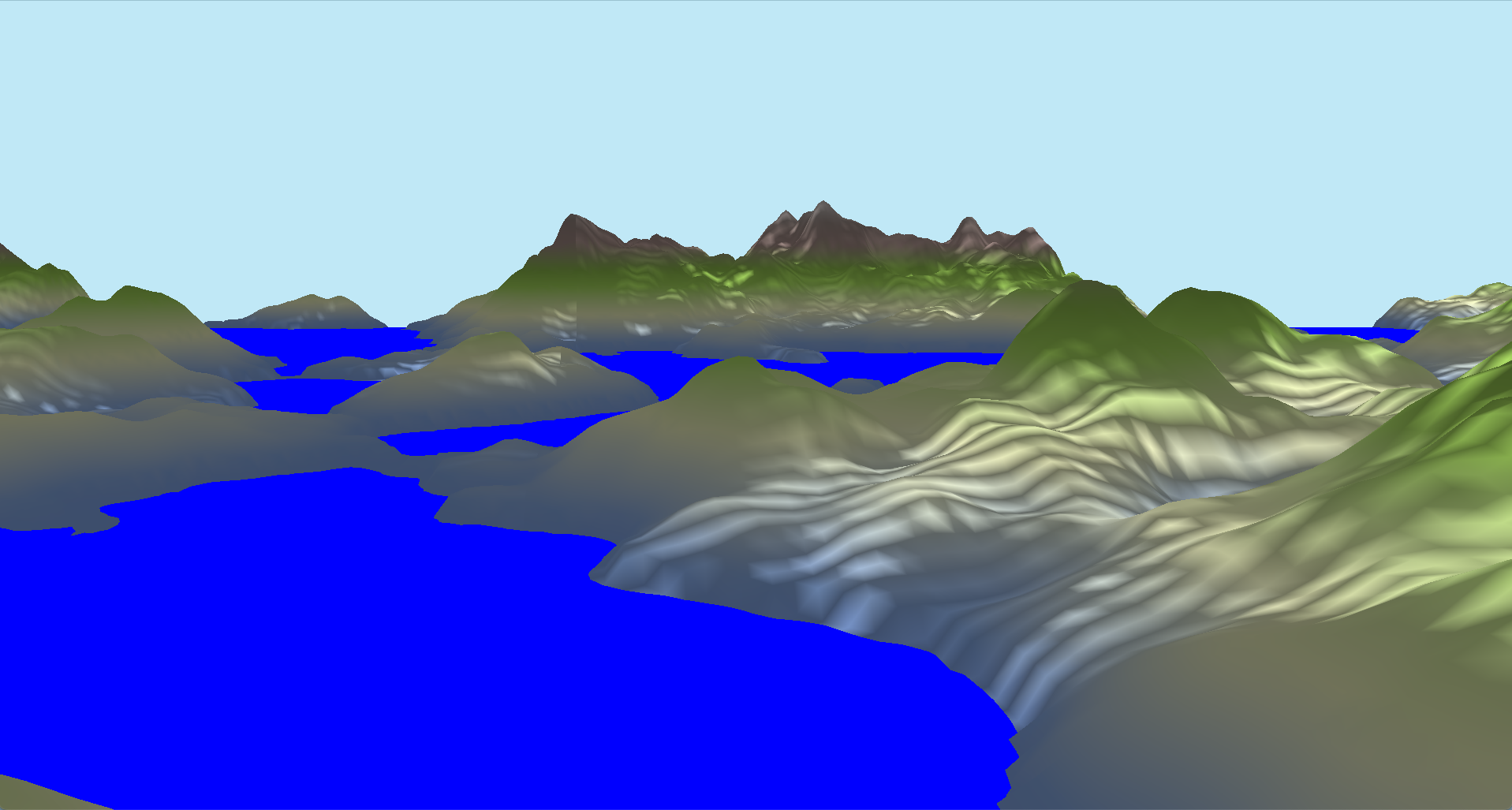
There were also issues with supporting how the terrain is rendered chunk-by-chunk. Vertices are defined locally to an origin (the center of a chunk) and thus an object-to-world coordinate matrix must be calculated. We adopt the original author's design, creating an array of Vertex Array Objects (VAOs) which hold the relevant chunk's water planes, and based on the index of the VAO, we calculate the corresponding transformation.
Z-fighting between the terrain and water plane was addressed by scaling down the heights of the terrain water vertices and increasing the heights of the rest of the vertices.
Texturing
With the water plane now set, we now move towards implementing the reflection and refraction effects on the water. This section and the next section of the water implementation follows this tutorial series by ThinMatrix , up to and including the Fresnel effect (varying refraction/reflection based on camera position).
The idea is that we create two additional Frame Buffer Objects (FBOs), separate from the default display. One FBO will correspond to reflections and the other will correspond to refractions — both will be used as textures. For the reflection texture, we reflect our camera along the axis of the water plane and render how the terrain and sky box appear. For our refraction texture, it will take the same rendering of the terrain as our display FBO. After rendering the transformed scene to each of these FBOs, we can use these renderings as a texture map for a water plane and achieve our desired effect.
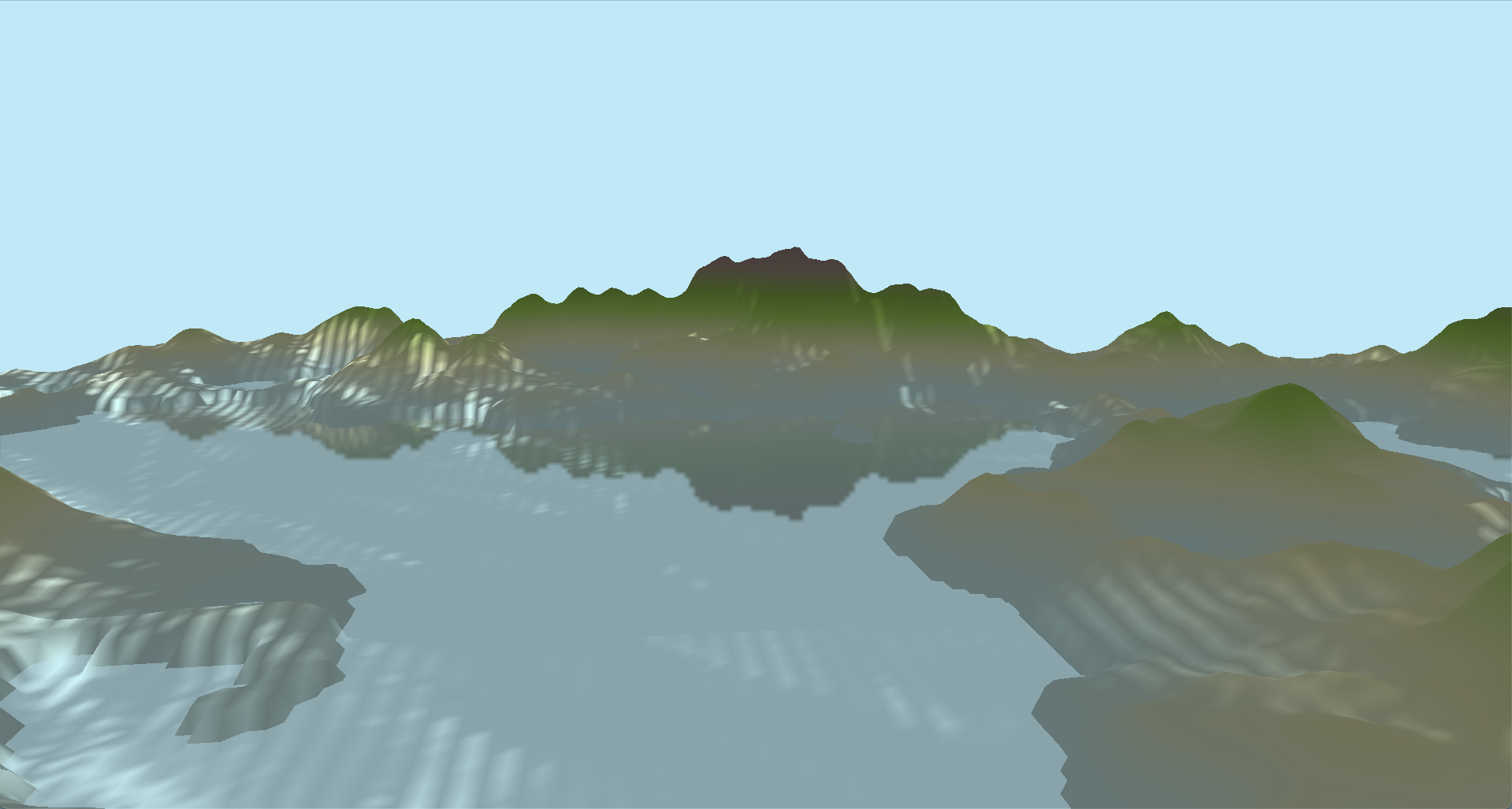
Distortion
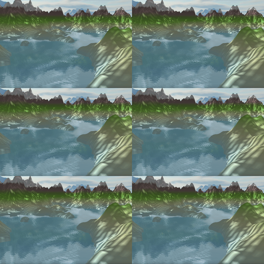
Lastly, we make the water more convincing by adding a distortion to the texture coordinates (for reflection and refraction), based on a dUdV map. To add movement, we can modify the distortion as a function of how many renders have occurred % 1.0, to cycle the movement.
With a little bit of finishing touches (and the cube map explained below), here's what we get!
Skybox
Our skybox implementation incorporates creating a cubemap and sampling pixels each of the different faces. For context, a cubemap takes in 6 individual images of a scene from the same fixed position but in 6 different directions. the field of view of these images is 90 degrees both horizontally and vertically and thus can get a scene in all directions. The 6 images are stitched together to create a single texture.
In our implementation, we first needed the 6 images of the skybox and we created a helper function to load them in and bind them to the proper texture target. Because a cubemap has 6 texture, we had to call glTexImage2D 6 times with their parameters set as well as telling OpenGL which side of the cubemap we are building the texture for. We also needed to set the wrapping method to GL_CLAMP_TO_EDGE because there may be a case where the texture coordinate is exactly between two faces. We then load the skybox as a cubemap with cubemapTexture as its id and finally bind it to a cube.
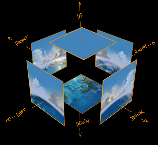
We then created a skybox shader that would sample the cubemap and render the skybox. We passed in the view and projection matrices to the shader and used the view matrix to remove the translation component so that the skybox would always be centered around the camera. We then used the projection matrix to project the skybox onto the screen and then sample the cubemap based on the direction of the camera and used the texture coordinates to get the color of the pixel. The input texture coordinate is teh world space coordinate of the vertex coordinates. Because our skybox is rendered behind everything else, we can do a trick where we render the skybox last and every pixel of the skybox has z-value of 1 so these pixels will draw to the buffer where there has not been a pixel drawn into it. Effectively, the skybox will draw where there isn't anything already drawn. To ensure that the z-value is always 1, we set z-value in clip space to be the same as the w-value because then when the vertices are converted into normalized device coordinates the x, y, and z coordinates are all divided by w.
In order to actually draw the cube, we will need another VAO, VBO, and a fresh set of vertices so we utilized a provided vertex data on LearnOpenGL. We needed to change the depth test to equal so that values equal to the depth buffer will also be overwritten. Next, because we do not want the camera to translate at all we will remove the translation section by taking the upper-left 3x3 matrix and convert it back into a 4x4 matrix.
Some difficulties we encountered as that sometimes the faces would be rendered but have dotted pixels instead of the actual texture. This meant the ordering of our textures were incorrect and needed to be adjusted. Other times there would be clear distinct lines in between the faces which meant the orientation of the faces were incorrect and the images needed to be rotated around.
Final Results
Here are some of the final results of our project:Fog Shading
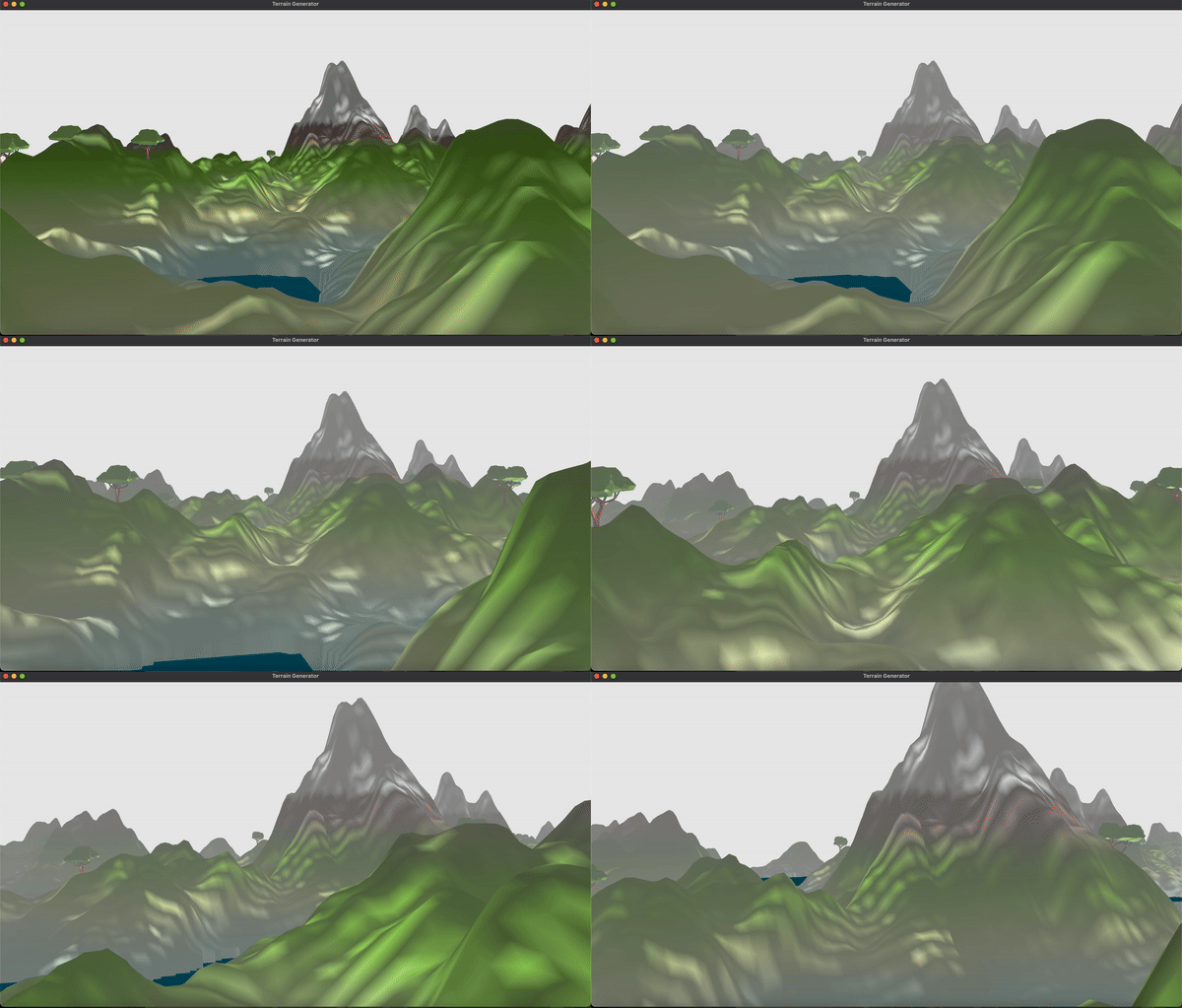
Here are some gifs of the fog shading in action. The first is linear fog, the second is exponential fog, and the third is exponential squared fog.


Grass Instancing
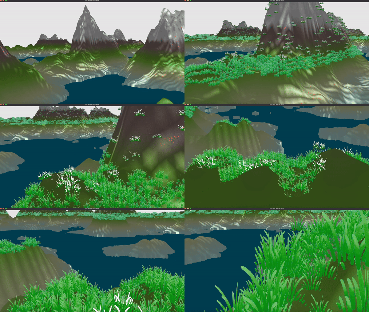
Here is a gif of the grass instancing in action. The grass is crisscrossed and the snowy grass is added on top.
Water Shader
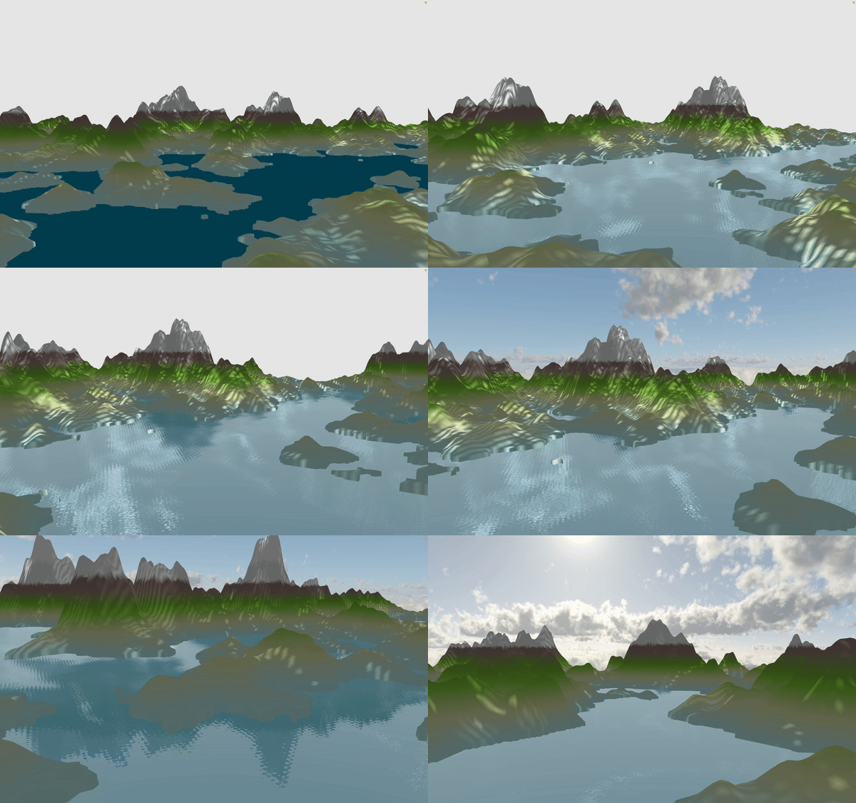
Here is a gif of the water shader in action. The water is reflective and refractive and has a distortion effect.
Skybox
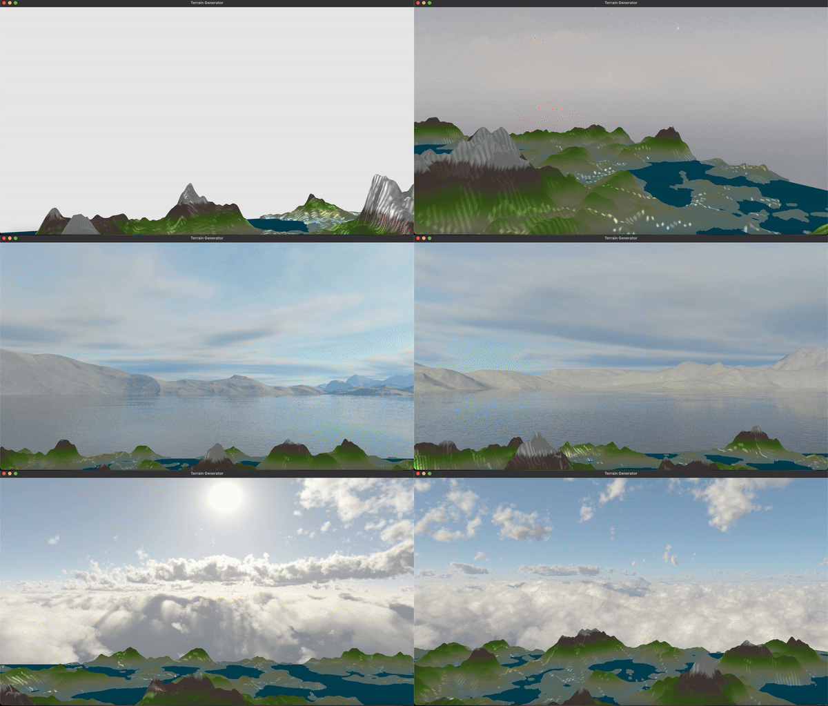
Here is a gif of the skybox in action with multiple different textures.
Final Presentation Video
Here is a video of our final presentation. We go over the different features we implemented:
Link to our slides can be found here.
References
- Atlas Github Repository by LiamHz
- Fog Shader Tutorial
- LearnOpenGL Shaders
- Grass Tutorial 1
- Grass Tutorial 2
- ThinMatrix Water Tutorial
- LearnOpenGL Cubemap Tutorial
- Skymap Tutorial 1
- Skymap Tutorial 2
Contributions
Ian
User Controls
- I helped set up some initial controls and added key bind toggles for each of the new shading that other team members implemented to see each of them separately and debug more efficiently.
- Ian tweaked the Perlin noise generation and set a random seed based on the date so that each time a new world would be randomly generated with different heights.
- Instead of showing individual triangles like the original project, Ian changed the flat colors so that each vertex would have their individual color and the triangle would have nicely interpolation and not all be a single color. Because the map would be colored based on the height, he decided to interpolate the colors to create a nicer blend between each triangle instead of having distinct sharp lines.
-
Ian implemented three different kinds of fog shading: linear, exponential, and exponential squared and smoothed
out the effects based on the distance from the pixel was away from the camera.
- Ian worked on creating a skybox through cubemapping to sample textures to create a 3D feel surrounding our terrain generated world. It helped create an illusion that the environment is way larger than it actually is.
Colin
Grass Instancing
- Colin helped get the initial repository set up and working on everyone's computer. Colin then added grass, which was a lot more work then it sounds (ha ha).
Zack
Water Shader
- Zack worked on implementing the water. He was responsible as well for grokking the rendering scheme of the initial codebase.
Satvik
Snowy Grass Instancing
- Satvik helped with getting the crisscrossing of 2D grass billboards to render. He also added snowy grass.